Version 2017-09-25
Simplified Modelling of Electric and Hybrid Vehicles
Massimo Ceraolo - University of Pisa
1 Introductory stuff
1.1 Acronyms
EHPT Electric and Hybrid Power Train
MSL Modelica Standard Language (in its rel. 3.2.2, except when otherwise specified)
MS Modelica specifications (in its rel. 4.3 except when otherwise specified)
1.2 Language and Tools
This chapter is written taking as reference MS 3.2 and MSL 3.2.2.
Since Modelica is a standard language, all Modelica-based models should in principle run with all the Modelica-capable tools. In practice this is not always true, and complex models cannot work in conjunction with some tool(s).
All the examples provided are checked with OpenModelica a very powerful open-source Modelica simulation tool, in its rel. 1.12.alpha1, 64bit Windows version.
OpenModelica is available for free, under different platforms (Windows, Mac, Unix) from its official site, http://www.openmodelica.org.
All the Modelica tool pictures included in this chapter are taken from OpenModelica. The appearance of that tool might slightly change from a computer to another, even running Windows, because the OpenModelica editor, OMEdit, is highly customisable, and my customization could have a slightly different appearance than readers .
Note that in this chapter we are not making usage of replaceable models, because these cannot be managed by the OMEdit GUI yet. This is not a big limitation: it just implies some additional replications of models. If this webbook has a future release, maybe replaceable components will be added, since this feature it is expected to be included in OMEdit in the coming months.
Once one has run a simulation using OpenModelica, the output can be analysed in other computers, even not having OpenModelica installed, especially if the CSV format is used an output. OpenModelica CSV outputs can be conveniently read and the result plotted and post-processed using the freeware PlotXY program, which can be downloaded from:
http://www.dsea.unipi.it/Members/ceraolow/Software/plotxy/plotxy-april-2014/view
Despite of what the pathname says, this program is continuously updated and the most recent version is dated 2017.
In this notebook, PlotXY has been used only whenever it is wished to have plotting functions that are not currently available in OMEdit, namely:
- plots with two vertical axes (useful for instance to show a current and a voltage or a torque and a speed agains time, each having its own vertical scale)
- parametric plots of more than one variable.
1.3 Model and data (txt) files
Before start the reader should have these files available: Download
wbEHVpkg.mo. It contains all the examples proposed in this chapter.
wbEHPTlib.mo. It is a support library necessary to run the examples in wbEHVPkg.mo.
Sort1.txt and NEDC.txt These are textual files containing two standard vehicular cycles: the Sort1 cycle and the NEDC cycle.
EVmaps.txt, SHEVmaps.txt and PSDmaps.txt contain numerical data (e.g. specific fuel consumption) for the engine and electrical drive used respectively in the MBEV example (sect. 3), SHEV examples (sect. 4.2 to 4.4) and PSD examples (sect. 4.5 to 4.8).
To make txt files them available in OMEdit, you have to put them in the OMEdit working directory. The location of OMEdit s working directory can be looked at, or set from the windows Tools|Options|General as shown below:
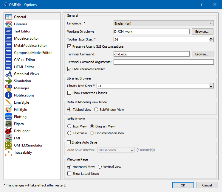
So, in the PC used to write this chapter this working directory is D:/OM_Work.
If the reader wants to change the numerical parameters of the models components he often will have to change them in the models dialog boxes. When the data are relatively a large number they are written in the above-mentioned text files (SHEVmaps.txt and PSDmaps.txt). So, to change the performance, e.g. fuel consumption, of the components the user has to change the data on these files. He can also have several text files related to different components and switch between them just changing the file name in the model s dialog box.
For instance:
If the user opens the genset dialog box of wbEvPkg.SHEV.SHEVpowerFiltSoc model, he will find that the default mapsfileName is SHEVmaps.txt . If he changes this name, the relevant ice data will be got from the file having the new name.
If the user opens the genset dialog box of wbEvPkg.SHEV.SHEVpowerFiltSocOO, he will find that the numerical data is not got from a file, but directly written in the dialog box. This is impractical, and one of this book s proposed activities is to modify this genset so that also its data are read from a txt file, in a way similar to that implemented in the SHEVpowerFiltSoc model.
If the user opens the ice dialog box of wbEvPkg.PSD.PSecu1 model, he will find that the default mapsfileName is PSDmaps.txt . If he changes this name, the relevant ice data will be got from the file having the new name.
If the user opens the gen dialog box of wbEvPkg.PSD.PSecu1 model, he will find that the numerical data is not got from a file, but directly written in the dialog box. This is impractical, and one of this book s proposed activities is to modify this gen so that also its data are read from a txt file, in a way similar to that implemented in the PSecu1 model.
1.4 Prerequisites to this chapter
This chapter is written having in mind a technical learner, typically an Engineering student at a bachelor level. Any learner that has at least the technical knowledge of a bachelor student in Engineering should be able to understand it easily. It could be also useful to any full engineer that wants to learn something about electric and hybrid vehicles, somehow hands-on . In fact Modelica offers learners an experience similar to the one we could have in a laboratory making tests on a full vehicle. With the advantage that we can measure everything without having to build complex measuring chains, and we can change everything in the physical and control parts of our system without having to spend a fortune, or risk an explosion.
Regarding Modelica, only some very basic experience with this language and MSL is required; one should be able to use a simulation tool, however. It is best if that simulation tool is the open-source OpenModelica (through the GUI interface offered by OMEdit), since all the pictures and the models presented are represented using OpenModelica s OMEdit.
1.5 About this chapter
Modelling of road vehicles is a highly multidisciplinary task. It may involve modelling with rotational mechanics, translational mechanics, electrical machines and converter, hydraulic components and systems, and more.
In particular, modelling electric and hybrid vehicles cannot absolutely avoid at least interfacing the electrical and mechanical domains, and their control.
Because of this, vehicle modelling and simulation in general, and electric and hybrid vehicle modelling in particular, are a field of engineering in which Modelica excels, because of its inherent capability to simulate multi-domain systems, from the ground up.
That is the rationale behind the choice of writing this chapter.
This chapter will not provide very detailed (thus huge) models, but instead models with a calibrated level of detail, which can help learning the basics and constitute a solid basis for building more compete and realistic versions of them.
2 My first EV model
The core of this chapter is simulation of EV s and HEV s power trains. All of the vehicle that is around the power train (chassis, auxiliary systems) will be dealt with only marginally.
A very basic representation of the vehicle s power train, using whenever possible MSL components and using a Modelica diagram, is in figure 1. It is a Modelica simulation model, according to MSL sect 1.2
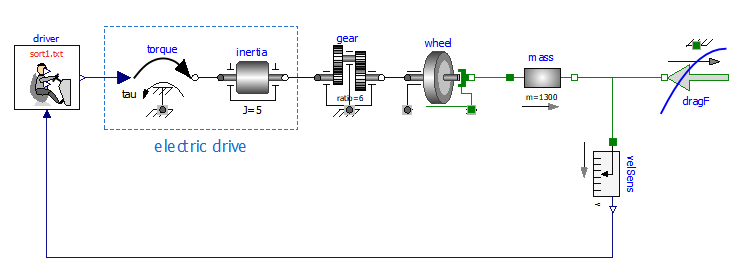
Figure 1. A first, very simple, EV Model.
Let us now explain the graphical elements (submodels of the simulation model in figure) shown, starting from its left side.
driver. It is impossible to simulate a vehicle without including in the simulation a driver model, unless we intend to consider a self-driving vehicle, which is totally out of the scope of this chapter. We will use a very simple driver model in this book, which are created on purpose, since they are not available in MSL. This driver model is described in section 2.4. It is designed to follow a kinematic drive, whose name is displayed in its icon ( Sort1.txt in the example above). It is a block, i.e a Modelica model without any physical connector, which generates signals that should be interpreted to be torque signal: accelerator (above), brake (below), combined (midrange, connected to power train in the figure above).
torque. This is the Modelica.Mechanics.Rotational.Sources.Torque. It plays the important role of connecting the cyber part of our simulation model to its physical part, in the direction cyber->physical; another connection between the two worlds, in the opposite direction, is made by the speed sensor at the right side of the picture above. The combination torque-inertia here simulates a power train that adds power to the signal issued by the driver. It could be for instance an electric drive, composed by an electronic converter and an electric motor.
inertia. This is the inertia of the electric drive, e.g. the rotational inertia of the rotor of an electric motor present in the power train.
electric drive. In this vehicle simplified model, the torque-inertia pair constitutes the electric drive, which receives as input a torque signal, positive when accelerating and negative when braking, and actuates it, considering the dynamics induced by the inertia. The electric drive absorbs or delivers power. This simple model does not show power conversion into electricity.
gear. Commonly EV s have only a fixed ratio reduction gear. That is the role of gear in the above picture.
wheel. This is an ideal rolling wheel. Note that in real-life cases wheels do not roll ideally. They have some slip, which is below 5% on good tyre-to-tarmac contact, and accelerations below 5-7 m/s2. Since this book describes simplified vehicle modelling and simulation, we always consider ideal rolling; the accelerations we will see will be, indeed, bell below the 5 m/s2 threshold.
mass. A very important part, though very simple, is the Modelica.Mechanics.Rotational. Components.Mass model called mass. It is the vehicular mass, in the example in figure 1400 kg. At its flange_a it is subject to propulsive force due to power train torque, at its flange_b to the resistance force to movement of the vehicle dragF.
velSens. As mentioned earlier, in terms of the cyber-physical simulation environment, which is Modelica, this sensor (as all sensors) creates a communication link between the physical and cyber parts of our simulation model. Looking at things in another way, it plays the role of a vehicle dashboard. The driver has in mind the kinematic cycle he wants to follow, and to do this he acts a closed-loop controller. Therefore, he looks at the actual speed through the dashboard (which in our mind displays the speed measured by velSens) compares it with the desired kinematic cycle, and acts on its commands (brake, accelerator) so that to reduce or nullify the error.
dragF. This an object describing the vehicle resistance to movement. Since this force requires some rather sophisticated code to avoid unexpected effects, this is not a MSL model. It is instead a model extended from Modelica.Mechanics.Translational.Interfaces. PartialFriction. A description of this model will be given in sect. 2.2
2.1 My first simulation: the Sort1 Cycle
I imagine the reader wishing to see our first simulation model at work, even before knowing all the details of its component models.
Therefore we introduce here a very simple driving cycle, which is able to show the basic characteristics of an electric vehicle motion. Although simple, the cycle were are going to introduce is standard. It is a standardised cycle used for urban bus testing, called Sort1 . Below you can see how this cycle is defined in a text file ( Sort1.txt ), its plot over time, and the resulting acceleration.
#1
# Standardised Sort1 cycle
# columns: time, speed (km/h)
double Cycle(13,2)
00.00 0.00
05.39 20.0
17.22 20.0
24.17 0.00
44.17 0.00
54.99 30.0
68.37 30.0
78.79 0.00
98.79 0.00
116.71 40.0
120.60 40.0
134.49 0.00
150.00 0.00
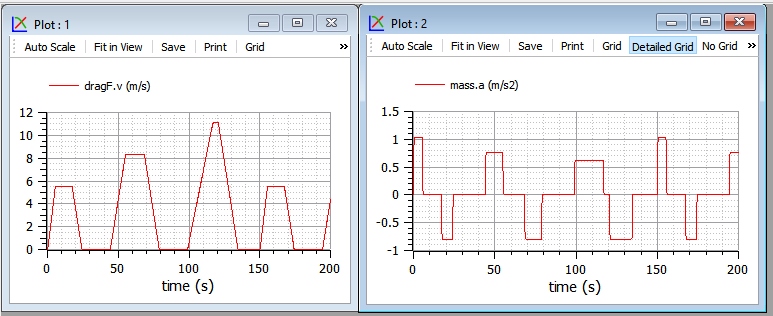
Figures 2. The sort1 cycle (left) and its resulting acceleration (right).
Note that these plots contain also the file name, so the reader can reproduce them by running the model with OMEdit, the GUI tool to use OpenModelica compiler.
To select a cycle in one of the supplied model, the reader has just to tell the driver the cycle name. E.g. for the sort1 cycle the driver s parameter window under OMEdit might appear as follows:
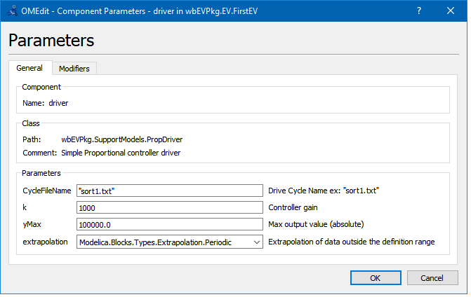
Figure 3. The parameter dialog box for the proposed driver model.
The Sort1 cycle, in its period which is 140s, has three trapezoids, which are scaled progressively: the acceleration reduces from the first trapezoid on, the maximum speed raises.
The above plots, as well as plots of many other quantities, can be obtained simulating an EV using the simulation model shown in figure 1, with the addition of two power sensors, giving rise to the model shown in figure 4. That model is available in the package wbEVPkg.mo under the name EV.FirstEVpow .
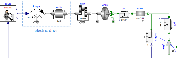
Figure 4: Model wbEVPkg.EV.FirstEVpow.
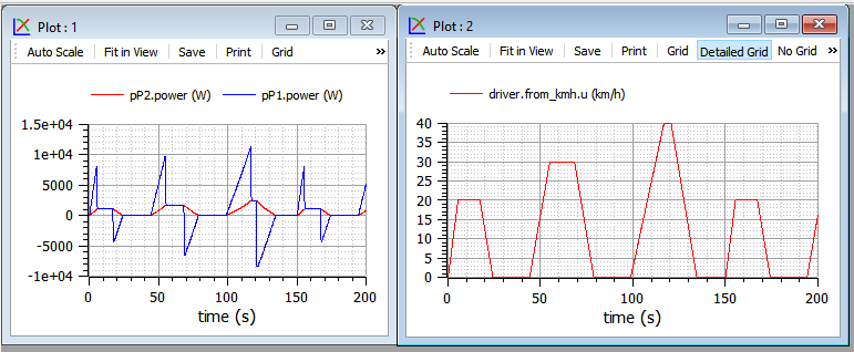
Figure 5. Powers and vehicle speed under the Sort1 cycle (model wbEVPkg.EV.FirstEVpow).
The same curves could be desplayed using twin vertical axes, but to do this we need to export variables as CSV and use and external programm, such as PlotXY, which is mentioned in the beginning of this notebook (and whose link is shown there). the apparance could be for instance as shown in figure 6.
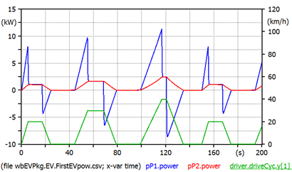
Figure 6. the same curves shown in ifugre 5, but using twin vertical axes.
Underlined varuables (here driver.driveCyc.y[1]) evaluated against the right vertical axis.
When speed is constant pP1 power equals pP2 s. During transients the two differ, and the difference is the accelerating torque. The areas between red and blue curves are kinetic energies: when the red curve is above the blue ones, we are accumulating kinetic energy in the vehicle s mass, when the position is reversed, that energy is given back to the power train. The power train shown in figure 5 is totally reversible and has no loss, i.e. it can be assumed to be an ideal EV power train since, in addition to not having losses, is able to fully recover braking energy. Therefore at the end of the simulation the net energy delivered by the electric drive is the area below red curve, which equals the area below the blue one (if we consider as initial and final two points in which vehicle speed is zero, i.e. time=0 and time=180s).
Drag force needs special consideration and will be discussed in the next section.
2.2 Details on DragForce model
According to vehicular mechanics, the resistance to movement force R for horizontal paths is usually expressed as follows:
R=fmg+1/2 SCx V2 (1)
The first term, containing the rolling resistance factor f, the mass m and gravity acceleration g, simulates rolling resistance; the second one simulates aerodynamic drag. In it, is the air density, S is the cross-sectional vehicle area, Cx the longitudinal drag coefficient, V the vehicle speed. Indeed using the (1) in simulations is incorrect; we must instead use the expressions shown in (2).
R=Fappl if V=0 and Fappl<fmg
R=fmg+1/2 SCxV2 otherwise (2)
This requires special code: when V crosses zero, it the vehicle is pushed with a force lower than fmg, it stays stuck at V=0. If instead of (2) we used (1) when the vehicle is standstill horizontally and no torque is applied to the wheel hubs, the vehicle would move backwards!
Note. When accelerating or braking the vertical load of front and real wheels are different from each other. For instance, when braking the load on front wheels is higher. The first term in (1) refers to the total load on the four wheels, whatever its distribution. This is correct whenever all the wheels are nearly rolling, that occurs in normal conditions, except when we have very high accelerations (e.g. more than 5-7 m/s2 on good tyre-to-tarmac contact). Therefore, the models in this chapter are valid if we avoid very strong accelerations, such that road-to-tarmac slips larger than 5-8% occur.
Equations (2) describe a behaviour that occurs whenever there is the switch from stationary grip to dynamic grip. E.g., in vehicles, in clutches and brakes. Therefore, a model for the dragForce able to operate correctly can be obtained using something already available in MSL.
The model wbEVPkg.SupportModels.DragForce is built slightly modifying Modelica.Mechanics. Translational.Components.Brake to introduce equations (2).
The reader could look at the whole code if he wants, but it is not very important. Here we just comment a few rows of code.
First we define protected parameters A and B as follows:
They are the two coefficients in equation (1)
Then we define the drag force, according to the R formulas in equation (2):
The part right of = is just copied from Translational.Components.Brake, without even try to understand all details. The part left of = is just equation (1), to which we added Sign that is the sign of V and considers whether the movement is forwards or backwards.
Finally, the brake model contains the variable free, which decouples the two brake parts when we are not braking. In our case this would occur when the considered wheel is not in contact with the asphalt, e.g. for a car jump . But our model is not able to simulate such things. We consider therefore wheels always in contact with the soil, and add the following row in DragForce:
2.2.1 Numerical values
In the simulations of section 2 as numerical values of the parameter connected to drag force we have used, and will be using the following ones, corresponding to a typical small car at typical air pressure:
m = 1300 kg, r=1.226 kg/m3, S=2.2 m2, f=0.014, Cx=0.26.
To see our dragForce at work, we can have a look at its flange force while still simulating the model shown in figures 1 and 5 (fig. 7).
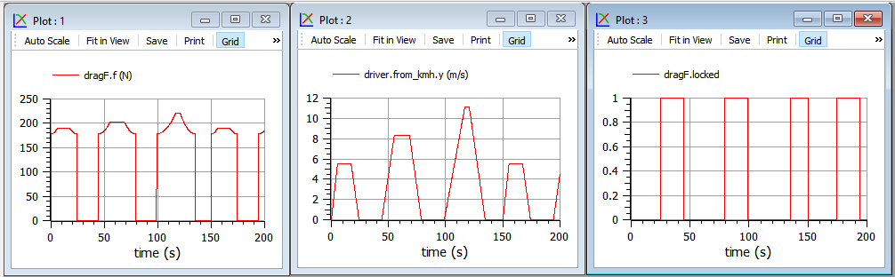
Figure 7. Drag force example, for a vehicle loperating under the Sort1 Cycle (model wbEVPkg.EV.FirstEV).
In the left plot we see that the part of drag force not depending on speed prevails, being around 180 N; while the part depending on speed becomes more and more significant when we move from the first to second and third trapezoid. This is reasonable, since typically in cars the aerodynamic part of drag force becomes prevalent starting from speeds around 80 km/h. With our parameters this critical speed is found from:
fmg=1/2 SCx Vcrit2
which gives Vcrit=81 km/h.
In the right plot we see two curves: the red one must be read on the left vertical axis and contains speed. The green one is a boolean variable indicating when the drag force understands the vehicle to be stopped, and its value is to be read on the right vertical axis (1 means true, 0 false). When locked=true the first of (2) is valid, otherwise the second one applies.
2.3 Simulating NEDC
NEDC (New European Driving Cycle) Cycle is richer than Sort1, and is thought for cars, not buses. It has an urban part, constituted each by three near-trapezoids, which is repeated four times, and a final extra-urban part.
To simulate this cycle the file name NEDC.txt must be chosen in the driver s parameter window, as shown earlier for Sort1 cycle. This cycle looks as in figure 8:
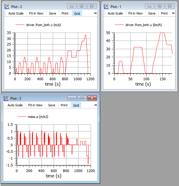
Figure 8. The NEDC cycle (top) and its resulting acceleration (bottom). Model wbEVPkg.EV.FirstEV.
To reproduce select NEDC.txt in driver's parameters dialog and use simulation time=1200s.
The acceleration plot shows very rapid acceleration changes even during ramps of the near-trapezoid shapes. These are due to the fact that this cycle was thought for conventional vehicles, in which during acceleration gears are switched, and during switching speed has a plateau (see zoom above) where acceleration goes to zero or so.
These plateaux are meaningless for EVs and those working with these vehicles usually use modified versions of the cycle hot having these plateaux.
A final note. NEDC cycle is very old. A new family of cycles has been developed as a worldwide effort, called WLTC (Worldwide Light-vehicle Test Cycles). They are planned to be progressively introduced in some countries, in particular in Europe, starting from September 2017 .
Also for the NEDC cycle the power plots as those in fig. 6 can be plotted, as per the following figure 9. Naturally actual powers depend not only on the kinematic cycle, but also on the vehicle parameters: mass, drag force. Also this figure is plotted with the external PlotXY program, since it contains two vertical axes. The reader is prompted to reproduce these curves using two separate plot windows in OMEdit.
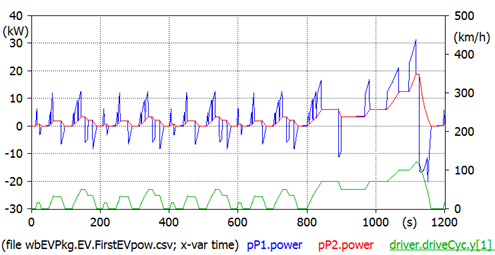
Figure 9. Some powers for a given vehicle operating under the NEDC cycle. Model wbEVPkg.EV.FirstEVPow.
To reproduce select NEDC.txt in driver's parameters dialog and use simulation time=1200s.
The peak power now reaches 30 kW inclusive of accelerating power, while the power needed to overcome motion resistance has a peak of 18.8 kW in the final part of the cycle, reaching 120 km/h.
2.4 Details of Driver model
The driver is a man, and therefore to simulate him models can be very complex. However, for our first EV, the driver has just to follow the given driving cycle, closely enough. In addition, this chapter is not to study people, but machines, i.e. our EVs and HEVs. Therefore, here a very simple driver model can be used. The driver model used is shown in the following figure:
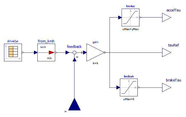
Figure 10. Proportional Driver model (wbEVPkg.SupportModels.PropDriver) diagram.
It is called PropDriver because it implements a simple proportional control. A real driver commands propulsion through acceleration and brake pedals. In a simplified way, we can say that a positive torque (i.e. so that the power train delivers power) is requested acting on the accelerator pedal, while a negative one is requested while acting on the brake. This is how the above PropDriver works. The two signals are also combined into a unique torque signal, named tauRef.
Considering the situation more in detail, we must say that in reality accelerator can require negative torque as well, when the foot is released with the vehicle running at a given speed. This occurs naturally in a conventional vehicle (internal-combustion engine based) since when gas is zeroed releasing the accelerator pedal, inner ICE losses cause a mild negative torque to be delivered. This natural behaviour helps smooth driving, since it allows moderate braking without requiring displacing a foot from a pedal into another. Therefore, it is replicated artificially in modern EV controllers.
Just as an example, we can consider the technique to perform this accelerator release braking similar to that published in [2].
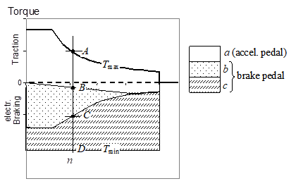
Figure 11. Operating regions showing a possible logic to manage pedal signals, and to get accelerator release braking.
According to that logic, an effective way of interpreting the driver commands, the zone between maximum and minimum electric drive torques Tmax and Tmin is split into three sub-zones in which the driver commands have different interpretations.
The zone a is limited by the upper part of the operating region and a straight line that passes in the point characterised by null torque and speed. At any generic Electric Drive speed n all points of segment AB correspond to different apertures of gas pedal position (GPP): for its maximum aperture, the maximum drive train torque Tmax is requested; for minimum aperture, a negative torque (then a light braking action) is requested whenever n>0; for intermediate apertures, linear interpolation is used.
Zone b (segment BC) is still available for stronger electrical braking action. Finally zone c (segment CD) adds mechanical braking.
Inside zone a there are parts with positive and part with negative torques. The latter realise the mentioned acceleration release braking. So, the position of the accelerator pedal totally released corresponds to zero torque only at the drive zero speed; that torque becomes negative at higher speeds to get moderate braking action.
When the user moves his foot to the braking pedal, in the first part of its span it will cover zone b, then zone c in which mechanical braking is added. This blending between mechanical and electrical braking can be obtained leaving in place the conventional hydraulic circuitry for mechanical braking, and exploiting the first part of the span for electric action. This is effective and leaves in place the current braking hardware, which is good to avoid safety reductions.
Practical implementation of this technique of interpreting driver s signals is not provided in the files provided along with this chapter. In them we will just use the combined torque signal tauRef in figure 10. Indeed evaluation of vehicle s performance can be done not going into this detail, as will be seen in the remainder of the chapter.
2.4.1 Proposed activity
The reader is prompted to modify the driver model as shown in figure 10, in such a way to implement the braking logic discussed in 11. The output to be connected to the torque input in figure 1 can still be the central output, which contains all torque requests; evaluation of accelTau and brakeTau, can be useful to evaluate the effects of the implemented accelerator release braking, and to fine-tuning it, e.g. counting the number of times in which the driver moves his foot from accelerator to brake pedals in several cycles, to try to reduce it to a minimum.
3 Map-based EV model
3.1 Introduction
The EV model used earlier was to understand the very basic behaviour of an EV power train, but has too many limitations for practical usage. In particular:
it does not consider any battery model and behaviour
it does not consider power train losses
it does not consider that braking can occur with either power train and mechanical brakes
it does not consider that power trains have limits in the torque and power they can deliver or absorb.
In the model presented in this section, we will remove these limitations. Nevertheless, they will not be very detailed for two reasons:
to understand things it is often better to have as simple models as possible
to allow simulation of the large time-spans required for vehicle simulations (minutes or tens of minutes) it is not wise to go into minute details such as commutation of valves inside vehicle power electronic converters.
The model we propose has the diagram shown in figure 12.
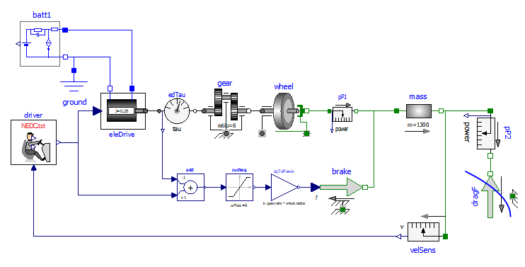
Figure 12: Map-based EV model diagram (Model wbEVPkg.EV.MBEV).
This model requires, to run, some data to be specified on a txt file. To reproduce the results shown here the reader can use the provided EVmaps.txt . How to link a txt file with a model is explained in section 1.3.
Some comments about the added components:
1. the battery model will be discussed in section 3.2
2. the drive train (eleDrive) model will be discussed in sect. 3.3
3. the brake action is simulated by just adding a braking force to the mass s flange_b. A more sophisticated brake model exists in MSL (Modelica.Mechanics.Translational.Components. Brake), but it was not chosen because in this book we prefer simplicity to completeness.
Regarding the above point 3, it is interesting to note that sum of torque is automatically made by any Modelica tool (here OpenModelica), since torque is a flow variable and flow variables are automatically algebraically summed up when several connectors are connected to each other. Here, the requested braking force is non-zero only when electric braking from eleDrive is insufficient.
Simulation of NEDC cycle using the model in figure 12 gives the results shown in the following pictures (fig. 13).
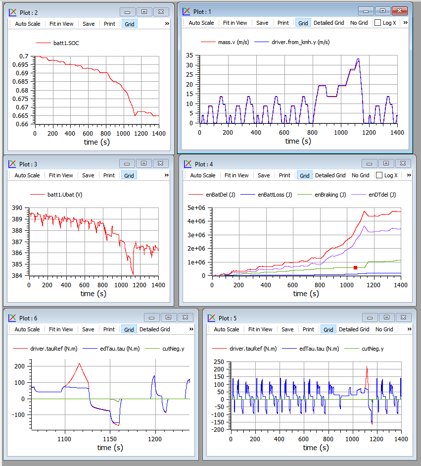
Figure 13. Plots related to the model in figure 12 operating under NEDC cycle.
Plot top-left contains the battery State-of-charge (SOC)
Plot top-right compares actual (red) and desired speed, and shows that they are very near to each other.
Plot middle-left contains the battery voltage
Bottom plots show torque request (red), torque delivered by the electric drive (green) torque corresponding to the mechanical braking force (blue). The left plot of the two is just a zoom on a section of the right one.
We can note that:
positive torques above 100 Nm are requested but not delivered. This is common in vehicles, whenever drivers request torques that are larger than maximum available, and in this case has no practical effects on the desired speed
negative torques are nearly always obtained with electric braking; mechanical braking here occurs only at the final deceleration of the extra-urban part (plot zoom in the lower right corner). In practice, however, real EV s use more mechanical braking. Compare with figure 43 in sect. 5.3.1
Plot middle-right shows energies. In this case energies are obtained using direct equation writing, to avoid the diagram to become too crowded. They are simply the following ones, in model MBEV:
Modelica.SIunits.Energy enBatDel, enDTdel, enP1del, enBattLoss;
equation
der(enBatDel) = (batt1.p.v - batt1.n.v) * batt1.n.i;
der(enDTdel) = driveTrain.powSensor.power;
der(enP1del) = mP1.power;
der(enBattLoss) = batt1.powerLoss;
The variable enDTdel is the energy delivered by the power train, while enP1Del is the energy supplied to the left flange of mass: the two powers differ from each other only when speed varies: the areas between the curves are the kinetic energy stored in driveTrain s inertia, and compensate to each other.
The total vehicle efficiency is not very high, due to the assumed efficiency map; finally the dark-red curve shows the energy lost inside the battery, in its inner resistance and other dissipation elements. To evaluate the battery cycle efficiency, however, it should first be recharged.
The model EleDrive in figure 12 is a component able to operate at a maximum permissible torque and maximum permissible power. These limits can be plotted in a torque-speed diagram, in which we can put also the points in which the vehicle operates under a given cycle. Figure 14 Contains a parametric plot showing the vehicle operating points under NEDC, inside the operating map.
It was drawn using a plotting program outside OMEdit (the program PlotXY mentioned at the beginning of this notebook), because currently OMEdit does not allow multi-curve parametric plots. Using outside programs is easy with OM, since it can save data as a CSV (Comma-Separated Values) file.
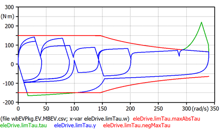
Figure 14. Actual torques (blue) shown inside the limits (red).
The red curves are the maximum and minimum allowed torques. The curve requested by the driver curve stays most of the time inside, and is shown in blue; when it should have gone beyond, it is cut and shown in green.
To reproduce these data the user has to:
- set "k" parameter in the driver model instance=100
- set max torque (tauMax parameter in eleDrive model) = 150 Nm
- set max power (powMax parameter in eleDrive model) = 22 kW
- use CSV as output file format for the whole simulation, or draw the preferred variables in a plot and export as a CSV file only them, sing the "Export Variables" tool-button in OMEdit (it shows as image "CSV" and a red arrow).
A typical EV study consists of the evaluation of the actual operating points (i.e. the points belonging to the green curve in the diagram above), in a diagram plan containing the map efficiency: in case they stay too often in zones having low efficiency, something must be changed in the power train design.
More on the efficiency maps in sect.5.
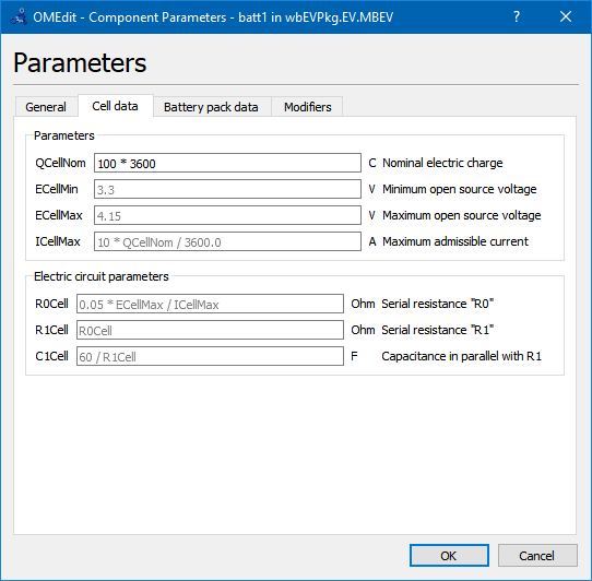
The dialog to introduce drive-train parameters is as in figure 15. Note that writing the efficiency map directly is not that practical. Therefore is written into a file. In the example provided the file is the provided EVmaps.txt and the variable name stored in that file is effTable .
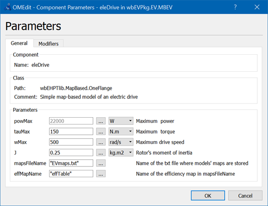
Figure 15. Dialog box to set parameter of eleDrive component (OneFlange class).
Just to be more explicit, the provided EVmaps.txt has the following aspect:
#1
# efficiency - rows:speeds pu, columns:torques pu
#
double effTable (6,6)
0.00 0.00 0.25 0.50 0.75 1.00
0.00 0.75 0.80 0.81 0.82 0.83
0.25 0.76 0.81 0.82 0.83 0.84
0.50 0.77 0.82 0.83 0.84 0.85
0.75 0.78 0.83 0.84 0.85 0.87
1.00 0.80 0.84 0.85 0.86 0.88
Note that the efficiencies in the file are with reference to values of rotational speed, p.u. of wMax and torque, p.u. of tauMax (see dialog box in figure 15).
It is interesting to evaluate the amount of energy recovered when braking, that would otherwise be lost. To do this, the model can be slightly modified in a graphical way, or with addition of the following code:
This braking energy is compared with pP1 energy in the plots in figure 16:
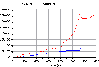
Figure 16. Braking Energy (green) compared with total energy (red) to vehicle mass
(model wbEVPkg.EV.MBEV).
3.1.1 Model limitations
The proposed EV model is simple and thought for teaching.
Many more additions could be made for industrial production models either in terms of completeness (e.g. some vehicles have switching gears, which is not included in our model), or accuracy: being map-based, this model is not able to depict the machine currents and other electric quantities in detail.
3.1.2 Proposed activity
Modify the wbEHPTlib.MapBased.OneFlange model in such a way that the efficiency map is loaded from file.
This can be done taking inspiration from the Driver s model, which already uses this technique.
Another useful activity is to modify MBEV in such a way that all braking energy is lost in brakes. This will be a better picture than that in figure 16 of the advantages of braking energy recovery.
3.2 Modelling batteries
Our battery model has the structure as shown in figure 17 that replicates, with additions (in red), our models icon. It is rather directly drawn from paper [1] which, published on 2000, has had a wealth of 274 citations and 4321 full text views since then , and many papers have appeared in subsequent years that replicated the approach used there. Although the original paper [1] referred to lead-acid batteries, that same model has proved to be adequate also for other kind of batteries, such as lithium based [5].
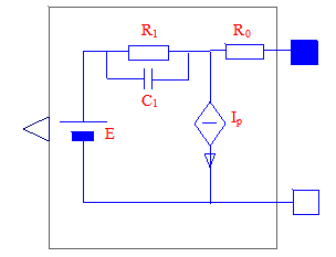
Figure 17. The icon of our battery model (wbEVPkg.SupportModels.Batt1)..
The model consists of an electromotive force E, an R-C network, a parasitic current Ip-The charge stored in the battery is the integral of current flowing through E, while the integral of Ip is charge that is lost.
In paper [1] E is a complex function of the battery state-of-charge SOC, and Ip is a function of battery voltage and temperature. However, this chapter is not a study about batteries. We can add here two simplifying hypotheses:
we take E as proportional to the stored charge. Therefore E itself can be substituted by a capacitor, having a very, very large capacitance, and a voltage equal to the so called open circuit voltage (OCV), i.e. the voltage that can be measured when the battery is disconnected from the outside circuit, and has stayed disconnected for a while. Therefore, that capacitor will still partially charged even when the battery is discharged.
Ip is taken as being a fixed fraction of the absolute value of the current flowing through terminals.
The diagram of the model we propose, is then as follows:
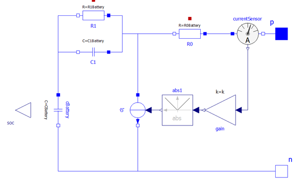
Figure. 18. The diagram of our battery model (wbEVPkg.SupportModels.Batt1).
Both internal capacitance cBattery and parasitic current Ip are automatically computed at initialization stage by the model itself, based on the user s data.
In this model, in fact, it is used the golden rule to ask the users, whenever possible, data in the form they are used to, and compute internally the data that are to be used during simulations. Below the tabs on the parameter window are shown.
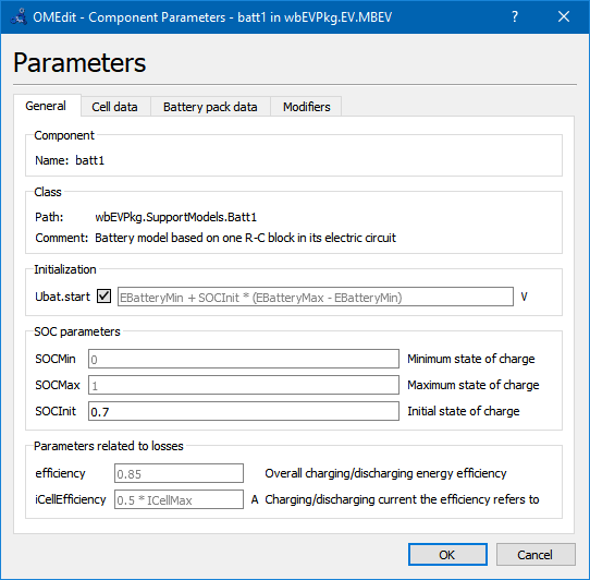
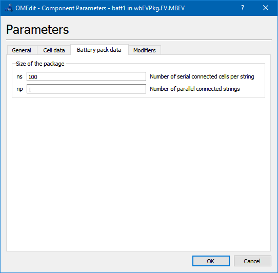
Battery pack data assume that the pack is made by parallel connection of np strings, each of which made up by a serial connection of ns cells.
The battery model gives as output the StateOfCharge SOC, defied by:
SOC=Qs/C=1-Qe/C (3)
where Qs is the stored charge , while Qe the extracted charge (starting from full battery). The definition involving Qe is more useful because the condition of battery full is more clearly defined than battery empty [1, 5]. However SOC is internally used in the model, the user may think of eq. (3) considering:
and tempty and tfull are time at which the battery is fully empty or full; and IE is the battery current entering its positive terminal.
The reader is however invited to have a look at the code to gain experience in reading Modelica code.
In one of the two the provided battery models, in addition to what shown here, a very small capacitance, named cDummy , has been added across the battery terminals. Being very small, this does not influence the results, but facilitates convergence in special circumstances.
3.2.1 Proposed activity
The reader could enhance the battery model substituting the capacitor with a SOC dependant EMF. He could first use a linear dependence, so that the behaviour of the fixed capacitor is reproduced. Then, a non-linear function, e.g. obtained using Modelica.blocks.Tables.CombiTable1D.
3.3 Map-based DC-interfaced electric drive
We already discussed the concept of map-based models. Our map-based model of an electric drive fed by a DC source is shown in figure 19 (wbEHPTlib.MapBased.Partial.PartialOneFlange).
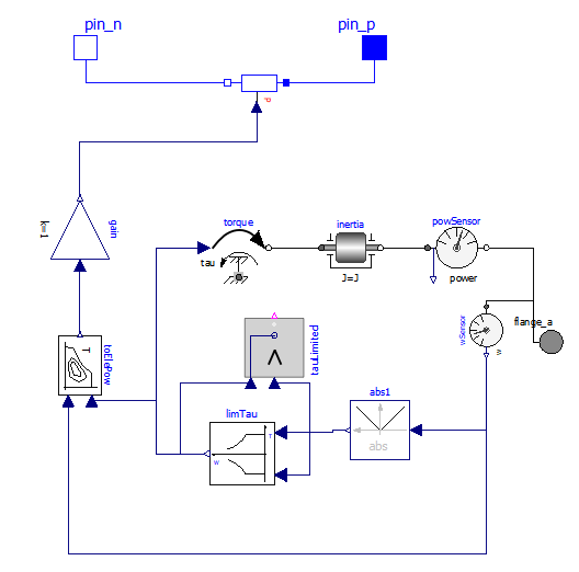
Figure 19. Diagram of the partial DC-interfaced Electric Drive model (wbEHPTLib.MapBased.Partial.PartialOneFlange).
Before discussing this model as a whole, the reader is prompted to have a look at the illustration of the utility blocks and models used here (blocks TauLim and EfficiencyT and model ConstPg), as found in sect 5.
Block limTau avoids the requested torque tau to overcome its maximum allowable; block toElePow computes the electric power from the mechanical inputs, considering the given efficiency map.
Finally the variable resistor model ConstPg at the top side of the picture, containing a red P, is an explicitly created model to interface map-based mechanical models with the corresponding electric circuit.
4 Map-based HEV models
4.1 HEV's resume
The reader is supposed to have some basic knowledge of what hybrid vehicles are and how they are structured. Therefore here we give just a brief resume.
According to ISO/TR 8713, a hybrid vehicle is a vehicle which has both a Rechargeable Energy Storage System (RESS) and a fueled power source for propulsion.
This corresponds to the following graphical representation:
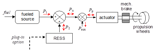
Figure 20. A general representation of a hybrid power train.
In which the red arrows indicate possible power directions. In the figure we use the following symbols:
P1: fuelled source power (positive)
P2: RESS power (positive when contributing to propulsion, negative when absorbing power into RESS)
Pu: useful power
Paux: power delivered absorbed by auxiliaries. In reality auxiliaries absorb power, so Paux is always a negative number as indicated by the red arrow. It is the sum of any load other than propulsion, e.g. lamps, GPS, radio, etc.
Pp: propulsion power: positive when in traction, negative when regen-braking.
The plug-in option is often provided to recharge RESS from the mains. This will not be considered in the remainder of this chapter.
We might say that the scheme in figure 20 is cyber-physical: the part left of the actuator is represented in terms of the block diagrams usually used to analyse control systems, and good at describing general fluxes, the part right of the actuator is more physical (it represents physical objects).
The scheme in figure 20 is rather general and accommodates several architectures. For instance, the fueled source could be an internal combustion engine (the most common case), a gas turbine, a fuel-cell generation system, etc. In this chapter we will only considered as fueled sources internal combustion engines.
Even while sticking to internal combustion engines, there are many ways in which this abstract representation can be implemented. Often they are classified as follows:
- Parallel Hybrid Vehicles (PHEV). Here there is a mechanical path from the ICE to wheels. Power contribution from RESS is added or subtracted to this main mechanical path
- Series Hybrid Vehicles (SHEV) Here the mechanical power produced by the ICE is first converted into electricity; then additional power from RESS is algebraically summed to this power, to generate the full propulsion power.
- Complex Hybrid Vehicles (CHEV): solutions which cannot be classified in the previous two architectures, e.g. in cases in which there is a parallel and a series power path.
In this chapter we present models of all these architectures. In the third group we choose a Power-Split-Device based architecture, which is the scheme used by the best-selling hybrid vehicle ever (the Toyota Prius that, according to [10], has sold between 1997-2013, over 3 million cars worldwide).
Note that since every HEV has two possible sources of electricity, there is an additional degree of freedom in comparison to conventional vehicles: at each time we can decide which part of the needed propulsion power is to be delivered by the fueled source, and which from the RESS.
Deciding this share is a complex operation since a lot of issues must be solved, related to the fact that the RESS can get discharged (and so cannot deliver power anymore), fully charged (cannot absorb power anymore), the load to be coped with, the useful power, is a function of time, the choices we make at a given time t influence what will happen in the future, and so on. This complex task is performed by a control system usually called EMS (Energy Management System), which takes as input the drivers commands and operates the power train in such a way to satisfy the propulsion and auxiliary power requests, while trying to maximise an performance index, typically the average efficiency (thus minimising the fuel consumption).
4.2 SHEV basic model
The SHEV model proposed here (wbEVPkg.SHEV.SHEVpowerFilt) has the following diagram:
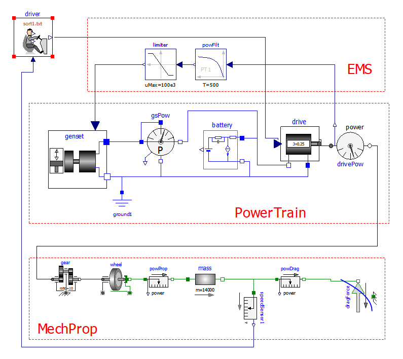
Figure 21 Diagram of the wbEVPkg.SHEV.SHEVpowerFilt model.
This model requires, to run, some data to be specified on a txt file. To reproduce the results shown here the reader can use the provided SHEVmaps.txt . How to link a txt file with a model is explained in section 1.3.
The lower part is the physical mechanical propulsion part used in the previous EV models.
In the central part of the picture the Power Train is detailed.
It contains a genset, which generates electricity, the battery batt, constituting the RESS in figure 20, a map-based electric drive drive of the same type used in section 3.
The upper port contains the EMS (whose need was discussed at the end of section 4.1), here having a very simple structure: it requires the genset to deliver the average propulsion power: in this way battery operates as a power filter : its delivers fast components of the propulsion power, leaving the average to the genset (i.e. the fueled source). Naturally, EMS must take into account the torque requests from the driver, which in turn tries to follow a given driving cycle, as seen when discussing pure (non-hybrid) electric vehicles.
Series Hybrids are most suited for urban trips, in which they allow important downsizing of the Internal combustion engine. Therefore here we test that hybrid using, as mass and resistance to movement data, numbers adequate for a bus: mass is 14 tonnes, cross sectional area 6 m2, Cx 0.65.
The following figure 22 shows some results, obtained when simulating a few repetitions of a Sort1 cycle that, as already noted, was conceived for buses. These results can be replicated simply by running wbEVPkg.SHEV.SHEVpowerFilt using the default data.
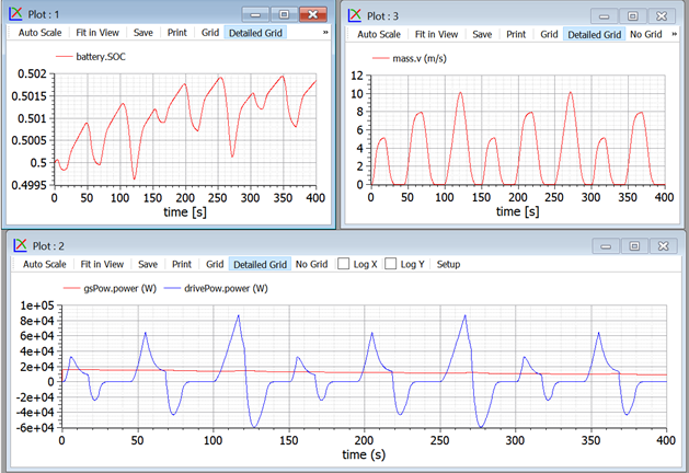
Figure 22. Plots of some Sort1 repetitions using the system in figure 21.
Note that the peak power required by this cycle is around 120 kW; using this hybridisation, the power required from the ICE is around only 7 kW.
The reader can reproduce these results selecting in the driver the Sort1 cycle as parameter.
However, buses, from time to time, are requested to cover also extra-urban routes, e.g. when going into the deposit at the end of the day or when they are to be transferred from a town to another.
Therefore it might be of use to evaluate also the performance of our hybrid bus also under the NEDC cycle.
This s easily done just changing the cycle (in the driver s parameter) and the simulation duration. Some results, which can obviously be reproduced by the reader, are as follows:
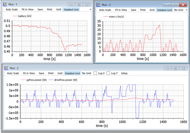
Figure 23. Plots of NEDC cycle using the system in figure 21.
In this case, powers, especially when the vehicle is in the extra-urban part, are much higher.
In addition, this simulation reveals a weakness of our model: the SOC drops significantly. This is because we ask the ICE to deliver the average power train power, as computed by a simple power filter. I.e., we have no correction factors for SOC departure from its reference value. The situation is improved in the next section.
4.3 SHEV with SOC closed-loop control
The problem of SOC control, shown in the previous section, can be addressed by adding in the EMS a correction term to the ICE requested power, according to the diagram of figure 24.
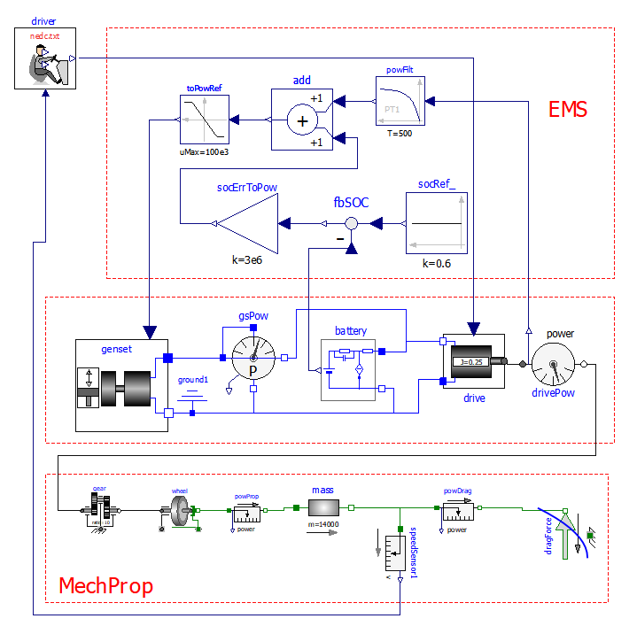
Figure 24: Diagram of the wbEVPkg.SHEV.SHEVpowerFiltSoc model
(Series Hybrid Electric Vehicles, with SOC control).
This model requires, to run, some data to be specified on a txt file. To reproduce the results shown here the reader can use the provided SHEVmaps.txt . How to link a txt file with a model is explained in section 1.3.
Some plots that can be obtained running the model whose diagram is in figure 24 are as follows:
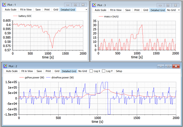
Figure 25. Plots of NEDC cycle using the system in figure 24.
Here, the SOC drops much less than the previous case, and continues to slowly recover, beyond t=1200 s, and go near to the reference set. The SOC set-point is socRef, the speed with which SOC is corrected to stay near the set point is the value of constant in socErrToPow.
4.3.1 Proposed activity
In case the bus has a plug-in architecture, it may be useful to discharge more the battery near the end of daily service, to take advantage of the cheaper mains recharge. This can be obtained by a driver command prepare for night , which changes the SOC set-point. Similarly, if the bus is allowed to go in a special city centre in EV mode (ICE shut-off), maybe the driver wants the battery to prepare for this run with a command prepare for ZEV .
The reader is prompted to modify the model giving this further level of control to the driver. Indeed in modern vehicles, in addition to accelerator and brake pedals, it is often possible for drivers to choose also the mode in which he want to drive (sports, economy, etc.) this additional command we are suggesting falls within the family of additional driver commands.
4.4 SHEV with On/Off control
In the model shown in the previous section, it has been noted that the ICE power is below 10 kW. The ICE size, however, is usually much larger than this, for instance to allow sustained driving at a motorway speed (e.g. 80 km/h) for instance during transfers to deposit or to another town (remember that our vehicle is a bus). With this requisite the ICE power should be at least 60 kW, as can be checked using equation (1) and possibly a constant-speed simulation with a high socErrToPow constant.
To allow some margin for acceleration, thus, a reasonable ICE sizing is a bit larger than 60 kW, say around 80-90 kW. With this size, however, during urban trips the ICE operates at a power that is less than one tenth of that size, which implies high specific fuel consumption. To enhance efficiency, an ON/OFF strategy can be envisaged: the ICE is switched OFF when the average power is too low, and for some time the vehicle operates taking all the propulsion energy from the battery. When the battery is partly discharged, the ICE is switched ON again, and works at a larger power since it has both to supply propulsion and recharge the battery.
Just to have an idea on how an ON/OFF strategy could look like and work, we can simulate the provided SHEVpowerFiltOO, which has the aspect shown in figure 26.
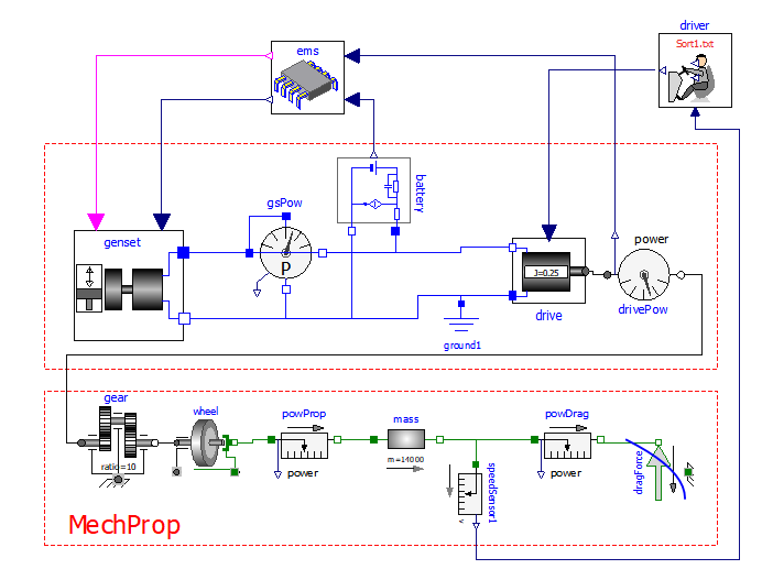
Figure 26: Model of the proposed Series Hybrid Electric Vehicles, with SOC control and ON/OFF.
This model requires, to run, some data to be specified on a txt file. To reproduce the results shown here the reader can use the provided SHEVmaps.txt . How to link a txt file with a model is explained in section 1.3.
The plots in figure 27 show some results with the Sort1 cycle (repeated many times, using for the driver the extrapolation Periodic ).
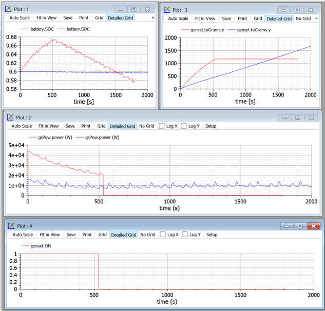
Figure 27. Comparison of SHEV behaviour with different control strategies
(SHEVpowerFiltSOC and SHEVpowerFiltSocOO, Sort1)
The consumption comparison can be made at t=1450s, where the two SOCs are equal to each other. In case of ON/OFF the engine is ON up to 520s, then OFF:
To reproduce these results, with the provided files, run SHEVpowerFiltSoc and SHEVpowerFiltOO. the socRef s used are 0.60 and 0.75 respectively; ON/OFF thresholds are 30 and 60 kW.
It is important to make these comparisons having care to consider times in which we have the same initial and final SOC, otherwise the results would been deceiving: we cannot fairly compare two simulations which exploit different quantities of the energy stored inside the battery.
The plots show that the ON/Off strategy makes the engine operate at powers near its nominal value, thus allowing better specific consumption.
4.4.1 Proposed Activity
In the previous section it has been seen that the proposed ON/OFF control reduces fuel consumption.
However the consumption depend on the switch-on and switch off thresholds chosen, and on the used cycle. In particular, the advantages are much more with Sort1 Cycle, which has a very low average power than with NEDC.
The reader is therefore prompted to change the cycle and the thresholds, to see their effect on consumption. Remember that comparisons are to be made at equal initial and final SOCs.
4.5 PSD-HEV model
While a SHEV can be considered a variation of a battery EV, with the addition of the fuelled source, a PHEV can be considered a variation of a conventional Vehicle, with the addition of an electric machine. In both cases, the smaller the addition, the nearer the vehicle to the original one (battery EV and conventional ICE based, respectively).
To create a simulation model of a PHEV therefore, we should start from a simulation of a conventional vehicle, with gears switching. This is not done in the current version of this model however, to reduce its complexity and length.
Instead, as an example of a general purpose hybrid vehicle, we will discuss a complex hybrid architecture, often called Series-parallel architecture, which is based on a planetary gears, called Power Split Device (PSD).
This architecture is installed on-board very successful commercial hybrid vehicles.
The implementation of this architecture we consider is shown in fig. 28. T s are torques, uppercase-omega s are angular speeds, P s are powers.
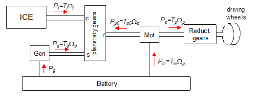
Figure 28. The considered PSD-based power train architecture.
The core of the power train is the planetary gears, which has an inner structure of the kind shown in figure 29.
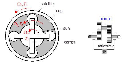
Figure 29 PSD (idealized) construction and corresponding MSL model (idealPlanetary).
It is nice to know that a planetary gear of this kind is already present in MSL. Its icon is shown in fig. 29 as well, in its right part.
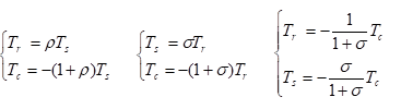
A simple analysis of kinematic and static relations of this device shows that two static and one kinematic equation exist. They can be expressed in different, equivalent forms. If we indicate with the ratio between ring and sun radius and with =1/ , we can equivalently write, as kinematic equations:

And as static equations:
Because of these relations, once one angular speed is known the PSD geometry determines the ratio between the other two; once a torque is knowns, the geometry of PSD determines the other two.
The above formulas are written according to the sign conventions used in MSL: torques are the torques acting from the outside towards the PSD, and the when they have the same sign as the corresponding angular speed, positive mechanical power is transferred from the outside towards the PSD.
In the architecture shown in figure 28 the internal combustion engine is flanged to the PSD carrier, the electric drive called generator Gen to the sun, the output shaft, to which the electric drive called motor, Mot is connected, to PSD s ring.
The architecture shown in figure 28 allows to choose the power to make flow in the battery, independently of the vehicle operation point. If this power is zero, we use a mode which we call electric balance mode, or CVT mode, since in this case we use the whole architecture as an intelligent Continuously-Variable Transmission (CVT). Otherwise, we can use some strategy to control the battery SOC, in a way similar to what done above with SHEV s.
Gen and Mot are reversible electric drives, since both can operate in motor and generator mode. However during vehicle traction and with all PSD speeds positive, Gen actually operates as a generator and Mot as a motor; the opposite occurs when, being the speeds still positive, the vehicle is regenerative braking and PSD output power is reversed.
In a way totally similar to SHEV basic model previously discussed now we show a logic in our PSD power train which tries to make the ICE deliver the average power needed for propulsion.
The principle diagram in figure 28 in our Modelica code becomes the diagram shown in figure 30.
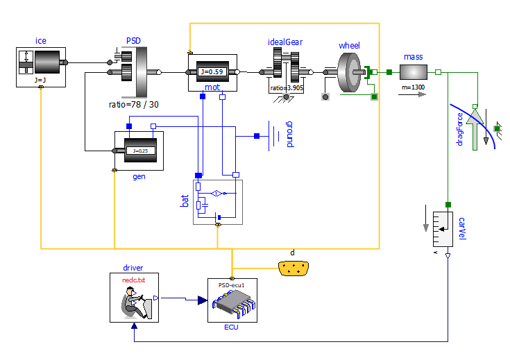
Figure 30. Modelica Diagram of the proposed PSD-based hybrid drive model (wbEVPkg.PSD.PSecu1).
This model requires, to run, some data to be specified on a txt file. To reproduce the results shown here the reader can use the provided PSDmaps.txt . How to link a txt file with a model is explained in section 1.3.
The reader should easily distinguish the elements in figure 28, with the addition of the control part, constituted by driver and Electronic control unit (ECU).
To reduce the wiring complexity, the various submodels signals are connected to each other by means of a bus (yellow).
To do this one has to:
1) decide with signals must flow in the bus and decide unique names since the various signals are distinguished by their name
2) create a specialised version of the various components, which are able to exchange their signals though expandable connectors, using the unique naming standard. The reader can easily see that the components in the above diagram are directly derived from the ones used above, with some modifications to allow connection though expandable connectors
3) create an Electronic Control Unit which manages the signals and implements the vehicle control logic.
The signals that will pass through our signal bus are listed in the following table:
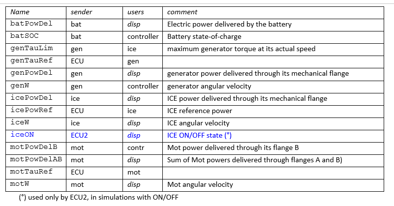
Several names are composed by two or three parts. The first part indicates the component to which the variable refers, (for instance "ice") the central one which kind of variable it is (for instance "tau" means torque), finally the(optional) third part indicates info about de variable for instance "del" means delivered, i.e. for a power a positive value indicates that the power is delivered to the outside by the component the variable belongs to; ref indicates a reference value (a variable that is used as a reference by some controller) Lim a limit, or maximum, value.
Jut to have an idea of the changes needed to make specialised, connector of components in the following figures we see first the component OneFlange, then its specific-connector-based version made with signal names related to PSD power trains, PsdGenConn.
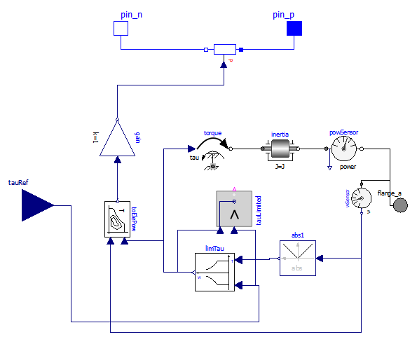
Figure 31. OneFlange model of an electric drive Input signal is reference tau tauRef
(wbEHPTlib.OneFlange).
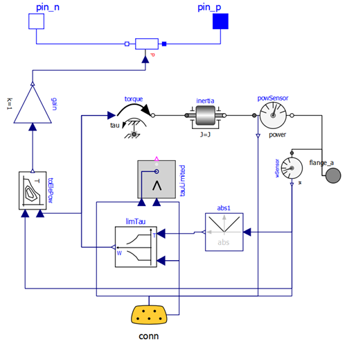
Figure 32. PsdGenConn Model of the generator machine of a PSD drive. It can be seen as a specialized version of the OneFlangeModel in figure 31, with a connector and signal names related to PSD generator.
The general arrangement is the same, but the torque reference instead of being taken from an input signal, it taken from the expandable connector, where it is called genTauRef.
Moreover, an additional signal is outputted, which can be exploited by any other model connected to the same bus, which is the mechanical output power and named genPowDel.
Now we will use the model whose gist has been described with three different control strategies, starting from the simpler moving towards the more complex.
4.5.1 ICE model
Our PSD model requires a map-based ICE model, not previously used. Our ICE model s diagram is shown in figure 33.
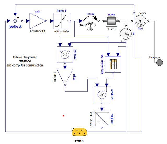
Figure 33. ICE model diagram (wbEHPTlib.MapBased.IceConnP)
The ICE dynamics is modelled by inertia; its fuel consumption by a map, read from a txt file (e.g. in the provided PSDMaps.txt). This model has a simple inner control logic, which tries to follow the input signal, sent through the expandable connector conn, containing a torque request.
Here, by simplicity, the maximum torque is limited by a constant value. More realistically, it should be limited using a variable limit, whose value is function of the rotational speed.
4.5.2 Proposed activity
The reader can enhance the supplied IceConnP model, making the maximum torque function of rotational speed. He can follow, as an example, the implementation of this kind of torque limitation used in the provided model wbEHPTLim.MapBases.ECUs.GMS.
4.6 PSD-HEV with power filter
Here we control the vehicle in such a way that the ICE delivers the average power needed for propulsion, and delivers it at its optimal speed, i.e. at the speed corresponding, for the given power, at the minimum fuel consumption. This logic implemented in the EMS, which has the scheme shown in figure 34.
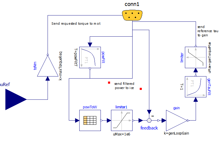
Figure 34. Diagram of ECU1 version of PSD-HEV Energy Management System (wbEHPTlib.ECUs.Ecu1).
In this scheme:
the received tau reference is sent back to connector as the signal motTauRef with just a scale adaptation. this way the motion control is attribute to mot, which is requested a torque directly depending on the torque request from the driver
to decide the power the ICE has to deliver, through conn, the propulsion power signal icePowRef is received, filtered through a first-order block, and the filtered back sent to ICE as a power request
the control of the ICE speed is attributes to the generator. Starting from the ICE power request, through the table powToW the corresponding optimal speed is determined, and used for a reference of a closed loop control, which determines the gen torque to be generated, genTauRef to try to obtain the wanted ICE speed.
It is ICE responsibility, through its inner control, to deliver the power the EMS requires. This is done inside the ICE block having the diagram shown in figure 33.
The reader is invited to perform the simulation of this model using the provided PSD.Psecu1 model. Just to give an idea of the result, some pictures are shown below:
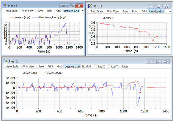
Figure 35 Some plots obtained when simulating the model in figure 30,
controlled with the ECU shown in figure 34 (ECU1) subject to NEDC cycle.
The plots show that the vehicle closely follows the requested NEDC cycle, with the ICE delivering (icePowDel) a smoothed version of the power needed for propulsion (icePowDelAB).
However, this is an open-loop control of the power that, in this case, causes a non-negligible shift in the battery SOC d.batSOC. In fact this cycle has a larger power request in its last part, the suburban section of the cycle, which is felt with delay by the averaging block, and never corrected.
Therefore it appears necessary to enhance the control logic, so that SOC is kept under better control.
4.7 PSD-HEV with power filter and SOC-loop control
To enhance the previous simulation, the EMS is modified as follows and called ECU2. Note that no other component has changed.
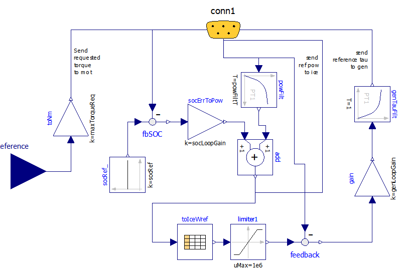
Figure 36. Modelica diagram of the proposed wbEHPTlib.ECUs.Ecu2 model.
A comparison with the diagram in figure 34 shows the difference: now the requested power is determined by the block add, which has two contributions: in addition to the previous one, consisting in the averaged propulsion power, we have a signal proportional to the SOC error.
The corresponding results are shown in figure 37.
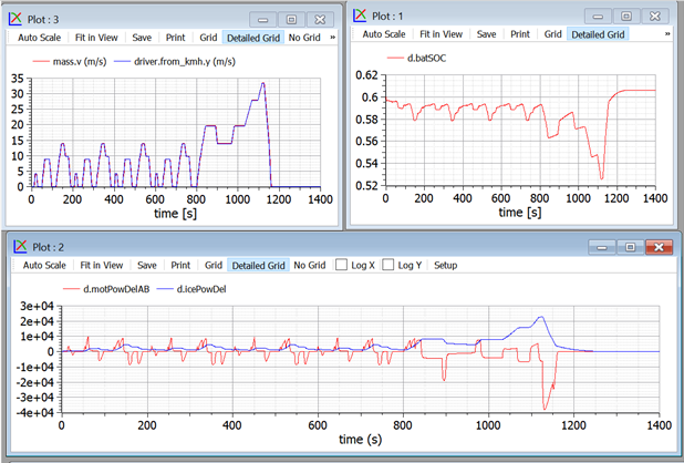
Figure 37. Some plots obtained when simulating the model in figure 30, controlled with the ECU shown in figure 36 (wbEVPkg.PSD.PSecu2), subject to NEDC cycle.
We see that now SOC is kept under much better control.
The control we implemented here is closely determined by the action of the two terms of the add block in Ecu2. We can enlarge or reduce the ice power and battery SOC fluctuations. With large values of the parameter powFiltT (the time constant in the block powFilt) and small values of parameter socLooopGain (the gain of the socToErrPow block) we will have a rather constant ICE speed, and large power and energy fluctuations in the battery, which needs to be sized accordingly. On the opposite side, smaller time constants of the power filter and large gains in the socToErrPow block will help keep the battery at a nearly constant level. In this case the battery can be smaller.
In extreme cases, we could design a vehicle with a very small battery, in which the propulsion power is nearly totally given by the ice, while during transients gen and mot supplied powers that are nearly one the opposite of the other (gen generates the power mot uses) to allow the PSD operating point to be changed, and the PSD architecture operates more like a Continuously Variable transmission than a true hybrid. This extreme choice, however, is not advisable since it would not leave room for regenerative braking.
To see these things in practice, the reader is advised not to tamper with ecu2 model directly, but, instead using its parameter dialog box, which has the following appearance:
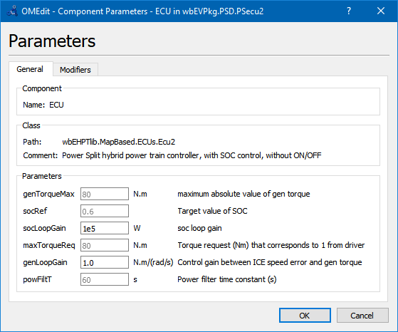
Acting on it, we change the value of the instance of ecu2 we use. The reader is prompted to do this while doing the following proposed activity.
4.7.1 Proposed activity
The proposed model is for teaching purpose and not for production. Therefore is not very robust.
However, starting from the working version, the reader is invited to play with socLoopGain and powFiltT in ECU2, to try to obtain the behaviour described in the comment just above here. In particular it is given the task to size the control so that a small battery (just around 500 Wh, e.g. 100 cells of the type used in our models but having 5 Ah nominal capacity) is sufficient to cover NEDC, with SOC staying between 0.2 and 0.8.
To avoid to enter into operating zones which create numerical difficulties, it is suggested to make small variations at each simulation and to save models which better the previous ones, before making additional attempts.
As an example we can show what happens with a small battery: 2Ah-100 cells, which means for a nominal voltage of 1.2 V 240Wh: a very small battery. Using this battery, powFiltT= 10s, socLoopGain= 20 kW and SOCinit=SOCref=0.6: we get the following curves:
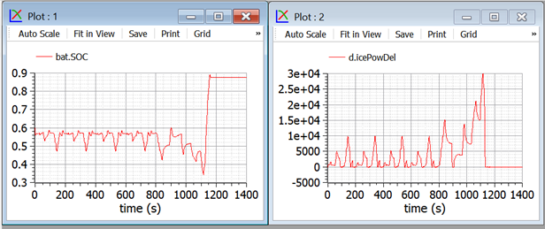
Figure 38. Some plots related to a small-battery proposed activity for PSD-hybrid.
In this case we privilege a small battery at the expenses of large ICE power variations.
Note that in the final part of our plots, when we have a strong braking action, the battery gest filled over the reference value of 0.6.
In case of even stronger braking, e.g. when running downhill, this small battery gets filled and part of the energy must be dispersed into heat using mechanical brakes.
Since mechanical braking is not present in the proposed models, if we try to further reduce the battery, during last braking the battery reaches SOC=1, and simulations stop since the power train can not brake anymore in absence of dissipative brakes.
4.8 PSD-HEV with power filter SOC control and ON/OFF
Consider the results shown in the previous section 4.7. From them, we see that on one hand, with the used battery size, battery SOC under NEDC varies a little; on the other during the urban part of it, the average power, which becomes the ICE power, is rather small, and therefore implies low ICE efficiency.
Because of this it is in this case advisable to envisage an ON/OFF strategy which automatically shuts-off the engine to avoid it to be too light loaded, in a way that is very similar to those seen for SHEV s.
To attain this control, a further modification of the EMS is made, giving rise to the Ecu3, whose diagram is shown in the following figure:
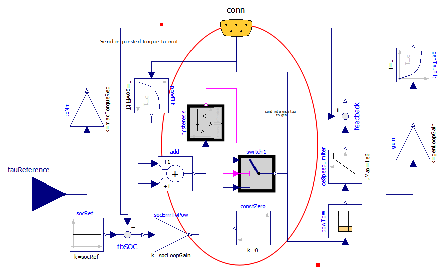
Figure 39 Modelica Diagram of wbEHPTlib.MapBased.ECUS.Ecu3.
Now the diagram has become rather complex, but the addition to the previous case is small, and highlighted with a circle.
ON/OFF is made through a hysteresis block, which switches the engine OFF when the power becomes lower than the lower threshold offThreshold and switches ON when the requested ICE power becomes larger than the higher threshold onThreshold.
Some of the results that can be obtained are summarised in the following picture.
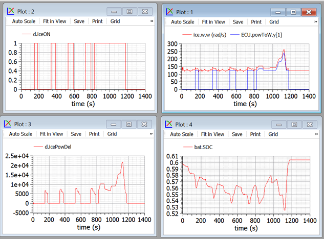
Figure 40. Plots from wbEVPkg.PSD.PSecu3 model.
It is easy to see that the ON/OFF strategy allows higher ICE powers when in ON state, and the SOC control is still guaranteed. The top-right picture shows that when ON the ICE operates near its optimal speed.
Ice is able to give information about the consumption in this case, compared with case in sect. 4.7.
This comparison must be made having the care of choosing control variables which allow to have in one case the battery more discharged than in the other, otherwise to comparison would be unreliable. So, to obtain the following pictures (fig. 41), some slight modifications on the control signals are made to obtain this SOC equivalence (ecu.SOCref, for the case with ON/OFF, changed to 0.65).
The results obtained playing with the supplied models are interesting, and showing below: the two simulations start at the same SOC, and reach the same SOC again for t= 1250. At this time the fuel consumed with ON/OFF is 0.356 kg, in comparison to 0.449 kg without it, implying a consumption reduction by over 20 %
It is reasonable to expect that using different thresholds the results can be even better. Naturally, for production usage, before deciding the ON/OFF thresholds several different cycles must be considered, while optimising on just a single NEDC is nearly a non-sense.
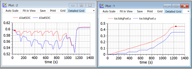
Figure 41 Fuel consumption comparison between non-ON/OFF and ON/OFF.
To replicate run wbEVPkg.PSD.PSecu2 and wbEVPkg.PSD.PSecu3 using the supplied parameters.
5 Map-based support models
5.1 EfficiencyT block
This block (the last T stands for table) having pathname wbEHPTlib.SupportModels. MapBasedRelated.EfficiencyT, receives as input a power train angular seed and torque, and outputs the corresponding power computed as the product of them, diminished by the internal losses evaluated by means of an efficiency map. Usually efficiency maps are known for families of components, in a normalised way. Because of this, a normalised map approach is used here as well. The diagram is as follows:
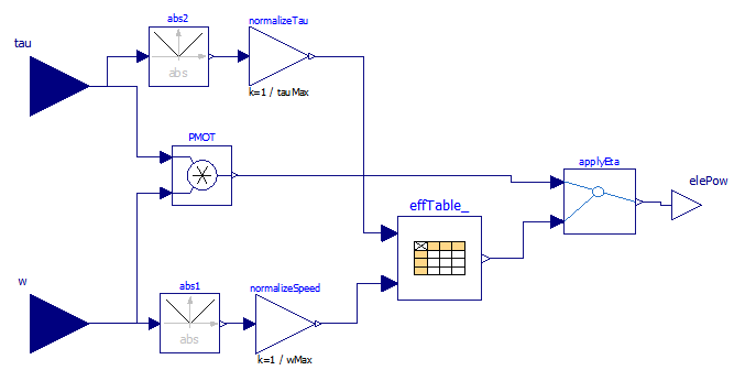
Figure 42 Diagram wbEHPTlib.SupportModels.MapBasedRelated.EfficiencyT block.
The model uses for the efficiency table a CombiTable2D component. That table can be used passing the matrix on-line or reading it from a file. In the provided form, it is passed on-line.
The numerical data inserted as an example in the model correspond to the following efficiency map, not drawn from a real case, but reproducing a somewhat reasonable trend.
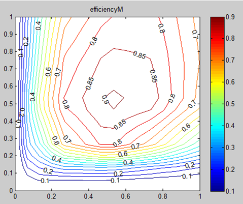
Figure 43. An example efficiency map
Drawing this kind of maps from numerical data is not a very easy task. If the user uses Scilab or Matlab, he can do this taking advantage of the contour() function.
The use of efficiency maps, though being very common and useful to graphically analyse things, has important drawbacks. The biggest difficulty is that on the horizontal and vertical axes (i.e. axes =0 and T=0) actual efficiencies hare zero, since mechanical power is zero, but losses are not zero. To use efficiency maps in MBEfficiencyT efficiencies on these axes cannot be set exactly to zero, to avoid division by zero, but to small values, e.g. 0.01. The map in figure 43 was drawn using exactly eff=0.01 on the axes.
Another way to introduce efficiencies in map-based models, is to introduce formulas to compute efficiencies. This is discussed in the next section.
5.1.1 Proposed activity
The reader is prompted to modify the model so that the effTable_ data are read from a file. The file name is to be passed as a parameter to the block.
5.2 MBEfficiencyLF block
This block (the last LF stands for Loss Formula) receives as input a power train angular speed and torque. In this case efficiency is computed through losses (fig 44).
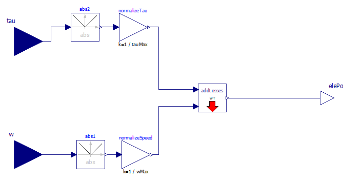
Figure 44. Diagram of the EfficiencyLF block.
Losses, in turn are computed through a loss formula (not a map, hence the model s name); addLosses has the following code:
Using the default parameters the obtained efficiency maps, respectively for traction and braking are as follows:
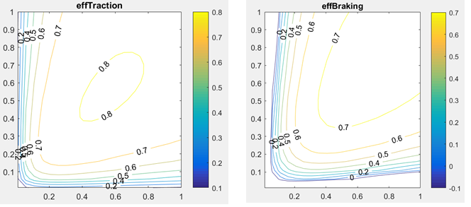
Figure 45. EfficiencyMaps with the proposed loss formula.
5.3 TauLim block
This block receives as input a torque request and measured speed; outputs the limited torque, i.e. the torque request if it is within limits, otherwise the maximum (or minimum) available torque.
The limiting torque is computed by limiting absolute value of power and torque as per the region shown in the model s icon, which is as follows:
Figure 46. Icon of the TauLimblock.
This is a typical simplified operating region of a drive train: it contains a maximum torque limit, a maximum power (the two hyperbolas), a maximum speed.
5.3.1 Proposed activity 1
The model tauLim has two significant limitations:
It considers only symmetrical curves around the horizontal axis, i.e. equal values for positive and negative limiting torques.
It does not consider automatic dropping of regions having negative efficiencies.
A more realistic map will have the shape shown in figure 47.
Figure 47. Improved torque limitation region.
In this figure not necessarily |Pmax|=|Pmin| nor |Tmax|=|Tmin|
Moreover a prohibited region , greyed, in present, where it is not convenient to operate the electric drive. In fact, in this region we can have negative efficiency. This is due to the fact that the mechanical power is lower than the electric losses to exchange that power. Instead of using that region, then, it is convenient to mechanical braking.
The code for TauLim included in the wbEHPTlib is very simple:
The reader is prompted to enhance this code, to give it more flexibility, allowing to generate a region of the type show in figure 47.
5.3.2 Proposed activity 2
This model is written for positive speeds. The user is prompted to modify it in such a way that it can operate also with negative speeds. The operating region therefore becomes four quadrant. In case this activity is done after Proposed activity 1, the improvements there made can be included also in activity 2.
5.4 ConstPg model
This model has the purpose to interface map-based mechanical models with the corresponding electric circuit. Its diagram is as follows:
Figure 48. Diagram of wbEHPTlib.SupportModels.MapBasedRelated.ConstPg.
It is based on a variable conductor, whose value is controlled so that the absorbed power equals the requested power, using a simple integral open.-loop controller.
It is very important to note that when this is connected to a real DC circuit, not always a solution can be found.
Consider, for instance that it is connected to a DC circuit which has a th venin equivalent with electromotive force Eth and inner resistance Rth. The situation is as shown in figure 49.
Figure 49. Duplicity of equilibrium point when a Thevenin DC source is loaded with a constant power load.
In the right part of the figure different load powers correspond to different hyperbolas. The green straight line correspond to the operating points compatible with the source DC circuit. It is apparent that beyond Plim no intersection exists between red and green curves, i.e. that power cannot be delivered. When P<Plim there exist two possible operation points, of which usually only the one with the higher voltage is acceptable.
This means that this kind of interface requires some attention that the requested power is not too much, and that the system initial condition is such that the wanted point (usually the upper one, as I said) is found by the solver.
Note that it is Plim=E2/(4Ri).
5.4.1 Proposed activities
1. The proposed model has as parameter the integrator constant. The provided formula contains also the nominal conductor voltage vNom. Why?
2. The integrator should have an initial value for output. Try to envisage which could be best and enhance the model to include this initial condition. Maybe a reference power pNom could be added as a parameter.
3. Try to insert the model in simple DC circuits to see where and when an operating point is found and when it is not. First you can use a circuit composed by fixed voltage in series with a fixed resistance. Then you can use more complicated circuits.
6 EV-HEV simulation concluding remarks
Specialised programs exist to simulate vehicle power trains (e.g. [9]). Also rich commercial libraries are available.
This chapter had not the ambition of discussing industrial-grade simulators. However, trough simple models, all based just on MSL, and progressive exercises, it hat the purpose to allow the reader to get to know the main issues and opportunities of simulating EVs and HEVs using Modelica and Open source simulators such as OpenModelica. At least OpenModelica and proposed models (all of which can be run through OpenModelica) are completely open, so one can understand, and modify, everything, up to the tiniest detail.
Indeed, in several occasions I felt that commercial programs, although powerful and reliable, have the important drawback of not allowing to understand all the details of the inner models.
Not always the more complex models are the best ones. For preliminary analyses, and evaluations, simpler ones allow to understand more easily the basic phenomena.
I hope that the reader that has got here has understood a lot regarding EV and HEV simulation, as well as HEV control and energy management.
7 References
[1] M. Ceraolo: New Dynamical Models of Lead-Acid Batteries , IEEE Transactions on Power Systems, November 2000, Vol. 15, N. 4, pp. 1184-1190.
[2] M. Ceraolo, A. Caleo, P. Capozzella, M. Marcacci, L. Carmignani, A. Pallottini: A Parallel-Hybrid Drive-Train for Propulsion of a Small Scooter , IEEE Transactions on Power Electronics, ISSN: 0885-8993, Vol. 21, N. 3, May 2006, pp768-778.
[3] M. Ehsani, Y. Gao, A. Emadi: Modern Electric, Hybrid Electric, and Fuel Cell Vehicles: Fundamentals, Theory, and Design , CRC Press, 2009, ISBN 9781420053982
[4] Toyota documentation http://www.evworld.com /library /toyotahs2.pdf, May 2003, file available for download on June 2017
[5] M. Ceraolo, T. Huria, G. Lutzemberger: Experimentally determined models for high-power lithium batteries , Book Advanced battery technology, ISBN: 978-0-7680-4749-3 doi:10.4271/2011-01-1365. Also presented at the SAE 2011 World Congress. Cobo Center Detroit, Michigan (USA), 12-14/4/2011.
[6] OpenModelica Consortium www.OpenModelica.org
[7] Dassault Syst mes Smart Electric Drives Library documentation: http://www.3ds.com/fileadmin/ PRODUCTS/ CATIA/ DYMOLA/PDF/dymola-smart-electric-drives-library.pdf; File available for download on April 2015
[8] Modelica Association: https://www.modelica.org/libraries, Vehicle Interfaces library Link available on April 2015.
[9] EERE Information Center, https://www1.eere.energy.gov/ vehiclesandfuels/pdfs/ success/ advisor_simulation_tool.pdf file available for download on June 2017.
[10] Information on Toyota unit sold from Toyota https://www.treehugger.com/cars/toyota-prius-hybrid-reaches-3-million-units-sold-worldwide.html
[11] Toyota Prius item on Wikipedia: https://it.wikipedia.org/wiki/Toyota_Prius